Introduction
A different error model can be defined for multiple endpoints models (eg. PK-PD, parent-metabolite, blood-urine…).
An example can be seen below, utilizing the warfarin data and model (provided by Tomoo Funaki and Nick Holford) from the nlmixr documentation (https://nlmixr2.org/articles/multiple-endpoints.html).
warfarin PKPD model
mod_warfarin_nlmixr <- function() {
    ini({
      #Fixed effects: population estimates
      THETA_ktr=0.106
      THETA_ka=-0.087
      THETA_cl=-2.03
      THETA_v=2.07
      THETA_emax=3.4
      THETA_ec50=0.00724
      THETA_kout=-2.9
      THETA_e0=4.57

      #Random effects: inter-individual variability
      ETA_ktr ~ 1.024695
      ETA_ka ~ 0.9518403
      ETA_cl ~ 0.5300943
      ETA_v ~ 0.4785394
      ETA_emax ~ 0.7134424
      ETA_ec50 ~ 0.7204165
      ETA_kout ~ 0.3563706
      ETA_e0 ~ 0.2660827

      #Unexplained residual variability
      cp.sd <- 0.144
      cp.prop.sd <- 0.15
      pca.sd <- 3.91
    })
    model({
      #Individual model and covariates
      ktr <- exp(THETA_ktr + ETA_ktr)
      ka <- exp(THETA_ka + ETA_ka)
      cl <- exp(THETA_cl + ETA_cl)
      v <- exp(THETA_v + ETA_v)
      emax = expit(THETA_emax + ETA_emax)
      ec50 =  exp(THETA_ec50 + ETA_ec50)
      kout = exp(THETA_kout + ETA_kout)
      e0 = exp(THETA_e0 + ETA_e0)

      #Structural model defined using ordinary differential equations (ODE)
      DCP = center/v
      PD=1-emax*DCP/(ec50+DCP)

      effect(0) = e0
      kin = e0*kout

      d/dt(depot) = -ktr * depot
      d/dt(gut) =  ktr * depot -ka * gut
      d/dt(center) =  ka * gut - cl / v * center
      d/dt(effect) = kin*PD -kout*effect

      cp = center / v
      pca = effect

      #Model for unexplained residual variability
      cp ~ add(cp.sd) + prop(cp.prop.sd)
      pca ~ add(pca.sd)
    })
}
data: first subject from the warfarin dataset
warf_01 <- data.frame(ID=1,
                      TIME=c(0.0,1.0,3.0,6.0,24.0,24.0,36.0,36.0,48.0,48.0,72.0,72.0,144.0),
                      DV=c(0.0,1.9,6.6,10.8,5.6,44.0,4.0,27.0,2.7,28.0,0.8,31.0,71.0),
                      DVID=c("cp","cp","cp","cp","cp","pca","cp","pca","cp","pca","cp","pca","pca"),
                      EVID=c(1,0,0,0,0,0,0,0,0,0,0,0,0),
                      AMT=c(100,0,0,0,0,0,0,0,0,0,0,0,0))
warf_01
#>    ID TIME   DV DVID EVID AMT
#> 1   1    0  0.0   cp    1 100
#> 2   1    1  1.9   cp    0   0
#> 3   1    3  6.6   cp    0   0
#> 4   1    6 10.8   cp    0   0
#> 5   1   24  5.6   cp    0   0
#> 6   1   24 44.0  pca    0   0
#> 7   1   36  4.0   cp    0   0
#> 8   1   36 27.0  pca    0   0
#> 9   1   48  2.7   cp    0   0
#> 10  1   48 28.0  pca    0   0
#> 11  1   72  0.8   cp    0   0
#> 12  1   72 31.0  pca    0   0
#> 13  1  144 71.0  pca    0   0
posologyr can compute the EBE for the combined PKPD model with
poso_estim_map()
map_warf_01 <- poso_estim_map(warf_01,mod_warfarin_nlmixr)
map_warf_01
#> $eta
#> ETA_ktr ETA_ka ETA_cl ETA_v ETA_emax ETA_ec50
#> -0.32297013 -0.54003647 0.79433822 -0.02976759 0.02346678 -0.28140889
#> ETA_kout ETA_e0
#> -0.30867037 -0.08384263
#>
#> $model
#> ── Solved rxode2 object ──
#> ── Parameters ($params): ──
#> THETA_ktr ETA_ktr THETA_ka ETA_ka THETA_cl ETA_cl
#> 0.10600000 -0.32297013 -0.08700000 -0.54003647 -2.03000000 0.79433822
#> THETA_v ETA_v THETA_emax ETA_emax THETA_ec50 ETA_ec50
#> 2.07000000 -0.02976759 3.40000000 0.02346678 0.00724000 -0.28140889
#> THETA_kout ETA_kout THETA_e0 ETA_e0
#> -2.90000000 -0.30867037 4.57000000 -0.08384263
#> ── Initial Conditions ($inits): ──
#> depot gut center effect
#> 0 0 0 0
#> ── First part of data (object): ──
#> # A tibble: 1,451 × 18
#> time ktr ka cl v emax ec50 kout e0 DCP PD kin
#> <dbl> <dbl> <dbl> <dbl> <dbl> <dbl> <dbl> <dbl> <dbl> <dbl> <dbl> <dbl>
#> 1 0 0.805 0.534 0.291 7.69 0.968 0.760 0.0404 88.8 0 1 3.59
#> 2 0.1 0.805 0.534 0.291 7.69 0.968 0.760 0.0404 88.8 0.0267 0.967 3.59
#> 3 0.2 0.805 0.534 0.291 7.69 0.968 0.760 0.0404 88.8 0.102 0.885 3.59
#> 4 0.3 0.805 0.534 0.291 7.69 0.968 0.760 0.0404 88.8 0.219 0.783 3.59
#> 5 0.4 0.805 0.534 0.291 7.69 0.968 0.760 0.0404 88.8 0.373 0.681 3.59
#> 6 0.5 0.805 0.534 0.291 7.69 0.968 0.760 0.0404 88.8 0.557 0.590 3.59
#> # ℹ 1,445 more rows
#> # ℹ 6 more variables: cp <dbl>, pca <dbl>, depot <dbl>, gut <dbl>,
#> # center <dbl>, effect <dbl>
#>
#> $event
#> id time amt evid
#> <int> <num> <num> <int>
#> 1: 1 0.0 NA 0
#> 2: 1 0.0 100 1
#> 3: 1 0.1 NA 0
#> 4: 1 0.2 NA 0
#> 5: 1 0.3 NA 0
#> ---
#> 1448: 1 144.6 NA 0
#> 1449: 1 144.7 NA 0
#> 1450: 1 144.8 NA 0
#> 1451: 1 144.9 NA 0
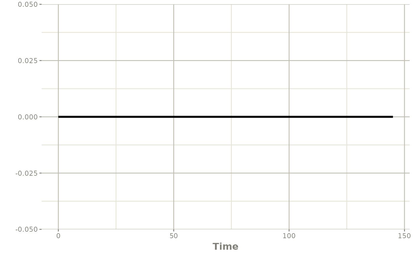
#> 1452: 1 145.0 NA 0The observation/time curves for both endpoints can also be plotted
plot(map_warf_01$model,"cp")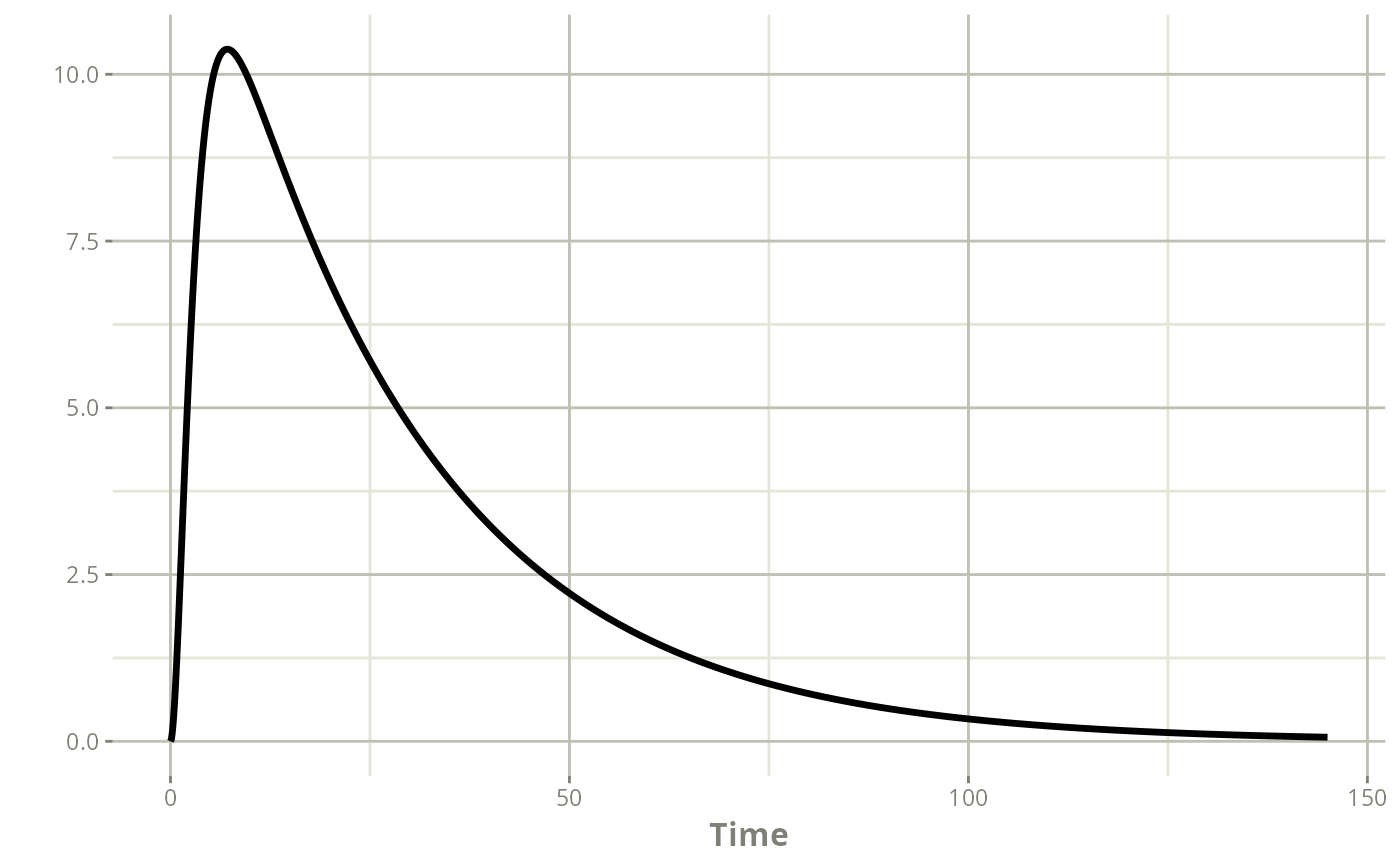
plot(map_warf_01$model,"pca")