Route of administration

library(posologyr)

Introduction

The Caldès 2009 ganciclovir model (https://doi.org/10.1128/aac.00085-09) is capable of describing the pharmacokinetics of either injectable ganciclovir or oral valganciclovir.

mod_ganciclovir_Caldes_2009 <- function() {
  ini({
    THETA_cl  <- 7.49
    THETA_v1  <- 31.90
    THETA_cld <- 10.20
    THETA_v2  <- 32.0
    THETA_ka  <- 0.895
    THETA_baf <- 0.825
    ETA_cl ~ 0.107
    ETA_v1 ~ 0.227
    ETA_ka ~ 0.464
    ETA_baf ~ 0.049
    add.sd <- 0.465
    prop.sd <- 0.143
  })
  model({
    TVcl  = THETA_cl*(ClCr/57);
    TVv1  = THETA_v1;
    TVcld = THETA_cld;
    TVv2  = THETA_v2;
    TVka  = THETA_ka;
    TVbaf = THETA_baf;

    cl  = TVcl*exp(ETA_cl);
    v1  = TVv1*exp(ETA_v1);
    cld = TVcld;
    v2  = TVv2;
    ka  = TVka*exp(ETA_ka);
    baf = TVbaf*exp(ETA_baf);

    k10 = cl/v1;
    k12 = cld / v1;
    k21 = cld / v2;
    Cc = centr/v1;

    d/dt(depot)  = -ka*depot
    d/dt(centr)  =  ka*depot - k10*centr - k12*centr + k21*periph;
    d/dt(periph) =                         k12*centr - k21*periph;
    d/dt(AUC)    = Cc;

    f(depot)=baf;
    alag(depot)=0.382;

    Cc ~ add(add.sd) + prop(prop.sd) + combined1()
  })
}

Intravenous ganciclovir

Patient record with TDM data

To describe intravenous administration, a CMT column has been added to the TDM data table to indicate administrations directly into the central compartment.

Note: to compute the AUC between the last dose and the time of the last dose + 24 hours, a dummy dose of 0 mg is added to the time of the last observation of interest (i.e. H144).

patient <- data.frame(ID=1,TIME=c(0,121,122,126,144),
                      DV=c(NA,10.8,5.8,3.3,NA),
                      ADDL=c(5,0,0,0,0),
                      II=c(24,0,0,0,0),
                      EVID=c(1,0,0,0,1),
                      CMT=c("centr",NA,NA,NA,"centr"),
                      AMT=c(250,0,0,0,0),
                      DUR=c(0.5,NA,NA,NA,NA),
                      ClCr=25)
patient
#>   ID TIME   DV ADDL II EVID   CMT AMT DUR ClCr
#> 1  1    0   NA    5 24    1 centr 250 0.5   25
#> 2  1  121 10.8    0  0    0  <NA>   0  NA   25
#> 3  1  122  5.8    0  0    0  <NA>   0  NA   25
#> 4  1  126  3.3    0  0    0  <NA>   0  NA   25
#> 5  1  144   NA    0  0    1 centr   0  NA   25

Individual PK profile and AUC 0-24

The individual PK profile can be estimated, and plotted.

map_patient <- poso_estim_map(patient,mod_ganciclovir_Caldes_2009)
#> using C compiler: ‘gcc (Ubuntu 11.4.0-1ubuntu1~22.04) 11.4.0’

plot(map_patient$model,Cc)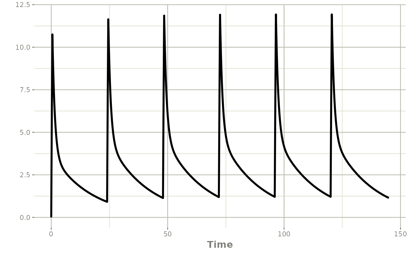

The difference between the cumulative AUC at H144 and that at H120 gives the AUC 0-24 after the last dose. Using data.table is optional, but the syntax is more convenient.

library(data.table)
data.table(map_patient$model)[time==144,AUC] - 
  data.table(map_patient$model)[time==120,AUC]
#> [1] 72.19085

Optimal dose for an intravenous ganciclovir injection

The optimal dose to achieve an AUC of 50 mg.h/L can be determined for a new injection of IV ganciclovir by setting cmt_dose = "centr".

poso_dose_auc(patient,mod_ganciclovir_Caldes_2009,tdm=TRUE,
              time_dose = 145,
              duration = 1,
              time_auc = 24,
              target_auc = 50,
              cmt_dose = "centr")
#> $dose
#> [1] 156.5335
#> 
#> $type_of_estimate
#> [1] "point estimate"
#> 
#> $auc_estimate
#> [1] 50
#> 
#> $indiv_param
#>   THETA_cl THETA_v1 THETA_cld THETA_v2 THETA_ka THETA_baf add.sd prop.sd
#> 1     7.49     31.9      10.2       32    0.895     0.825  0.465   0.143
#>       ETA_cl     ETA_v1        ETA_ka       ETA_baf covar
#> 1 0.05256541 -0.4773341 -3.589527e-08 -1.272466e-07    25

Optimal dose for an oral valganciclovir administration

The optimal dose to achieve an AUC of 50 mg.h/L can be determined for an administration of oral valganciclovir by setting cmt_dose = "depot".

poso_dose_auc(patient,mod_ganciclovir_Caldes_2009,tdm=TRUE,
              time_dose = 145,
              time_auc = 24,
              target_auc = 50,
              cmt_dose = "depot")
#> $dose
#> [1] 193.1298
#> 
#> $type_of_estimate
#> [1] "point estimate"
#> 
#> $auc_estimate
#> [1] 50
#> 
#> $indiv_param
#>   THETA_cl THETA_v1 THETA_cld THETA_v2 THETA_ka THETA_baf add.sd prop.sd
#> 1     7.49     31.9      10.2       32    0.895     0.825  0.465   0.143
#>      ETA_cl     ETA_v1        ETA_ka      ETA_baf covar
#> 1 0.0525648 -0.4773328 -1.018546e-06 2.327066e-07    25

Keeping the default value of cmt_dose, which is the first compartment declared in the PK model, would also work here.